放送大学「心理統計法(‘17)」第4章 生成量と研究仮説が正しい確率
- 授業ではRスクリプトを使ってますが、以下はPython3スクリプトです。
Python3のスクリプト
#!/usr/bin/env python3
# -*- coding:utf-8 -*-
import pickle
import hashlib
import os
import pystan
import numpy as np
import matplotlib
matplotlib.use('Agg')
import matplotlib.pyplot as plt
from os.path import basename, dirname
from scipy.stats import norm
#表1.1の「知覚時間」のデータ入力
data = [31.43,31.09,33.38,30.49,29.62,
35.40,32.58,28.96,29.43,28.52,
25.39,32.68,30.51,30.15,32.33,
30.43,32.50,32.07,32.35,31.57]
model_code = """
data {
int<lower=0> n; //データ数
real<lower=0> x[n]; //データ
}
parameters {
real mu; //平均(範囲指定)
real<lower=0> sigma; //標準偏差(範囲指定)
}
transformed parameters {
}
model {
x ~ normal(mu,sigma); //正規分布
}
generated quantities{
real xaste;
real log_lik;
xaste = normal_rng(mu,sigma); //予測分布
log_lik =normal_lpdf(x|mu,sigma); //対数確率
}
"""
def model_cache(model_code, path='./tmp'):
if not os.path.exists(path):
os.makedirs(path)
hashname = hashlib.md5(model_code.encode('utf-8')).hexdigest()
filename = '%s/%s.pkl' % (path, hashname)
if os.path.exists(filename):
with open(filename, 'rb') as fp:
model = pickle.load(fp)
else:
model = pystan.StanModel(model_code=model_code)
with open(filename, 'wb') as fp:
pickle.dump(model, fp)
return model
if __name__ == '__main__':
np.random.seed(1234) #乱数の種
model = model_cache(model_code)
fit = model.sampling(data={ 'x': data, 'n': len(data) }, chains=5, iter=2100, warmup=1000, thin=1)
print(fit)
pdata = fit.extract()
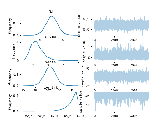
fit.plot()
plt.savefig("%s/%s1.png" % (dirname(__file__), basename(__file__)), dpi=90)
#plt.show()
sigma = pdata['sigma']
mu = pdata['mu']
xaste = pdata['xaste']
var = sigma**2 #分散(variance)
cv = sigma / mu #変動係数(coefficient of variation)
prob = np.array([0.025, 0.05, 0.5, 0.95, 0.975])*100
desc = [ "", "EAP", "post.sd" ] + prob.tolist()
varinfo = [ "分散 ", np.mean(var), np.std(var) ] + np.percentile(var, prob).tolist()
cvinfo = [ "変動係数", np.mean(cv), np.std(cv) ] + np.percentile(cv, prob).tolist()
fmt = "{:^18}" + "{:>10.2f}" * (len(varinfo) - 1)
print("")
print(("{:^8}{:>10}{:>10}" + "{:>9.1f}%"*(len(varinfo)-3)).format(*desc))
print(fmt.format(*varinfo))
print(fmt.format(*cvinfo))
es_refp = 30.0 # 効果量の基準点 (測定値で指定)
effs = (mu - es_refp) / sigma
effsinfo = [ "効果量(%d)" % es_refp, np.mean(effs), np.std(effs) ] + np.percentile(effs, prob).tolist()
print(fmt.format(*effsinfo))
pc_refp = 0.25 # %点の基準点 (下からの確率で指定)
pers = mu + norm.ppf(pc_refp) * sigma
persinfo = [ "%%点(%0.2f)" % pc_refp, np.mean(pers), np.std(pers) ] + np.percentile(pers, prob).tolist()
print(fmt.format(*persinfo))
upper = 30.5 # 分布関数上限 (測定値で指定)
lower = 29.5 # 分布関数下限 (測定値で指定)
mvs = norm.cdf(upper, mu, sigma) - norm.cdf(lower, mu, sigma)
mvsinfo = [ "測定値が%0.1fより大きく%0.1fより小さい確率" % (lower, upper), np.mean(mvs), np.std(mvs) ] + np.percentile(mvs, prob).tolist()
print(fmt.format(*mvsinfo))
mv_refp = 30.0 # 測定値との比の基準点(測定値で指定)
mvr = xaste / mv_refp
mvrinfo = [ "基準点との比(%d)" % mv_refp, np.mean(mvr), np.std(mvr) ] + np.percentile(mvr, prob).tolist()
print(fmt.format(*mvrinfo))
avg = 30 # 平均値がavgより小さい確率(測定値で指定)
print("平均値が(%0.1f)より小さい確率%10.2f" % (avg, np.mean(mu<avg)))
print("測定値が(%0.1f)より大きく(%0.1f)より小さい確率(点推定)%10.2f" % (lower, upper, np.mean((xaste>lower) & (xaste<upper))))
prob = 0.5
es = 30.0
print("(%0.1f)による効果量が(%0.1f)より小さい確率%10.2f" % (es, prob, np.mean((mu - es)/sigma<prob)))
prob = 0.2
mv = np.mean(norm.cdf(upper, mu, sigma) - norm.cdf(lower, mu, sigma) > prob)
print("測定値が(%0.1f)より大きく(%0.1f)より小さい確率が(%0.2f)より大きい確率%10.2f" % (lower, upper, prob, mv))実行の結果
Gradient evaluation took 1.1e-05 seconds
Gradient evaluation took 1.1e-05 seconds
Gradient evaluation took 1.2e-05 seconds
Gradient evaluation took 1.2e-05 seconds
1000 transitions using 10 leapfrog steps per transition would take 0.11 seconds.
1000 transitions using 10 leapfrog steps per transition would take 0.11 seconds.
Adjust your expectations accordingly!
1000 transitions using 10 leapfrog steps per transition would take 0.12 seconds.
1000 transitions using 10 leapfrog steps per transition would take 0.12 seconds.
Adjust your expectations accordingly!

Adjust your expectations accordingly!
Adjust your expectations accordingly!


Iteration:    1 / 2100 [  0%]  (Warmup)
Iteration:    1 / 2100 [  0%]  (Warmup)
Iteration:    1 / 2100 [  0%]  (Warmup)
Iteration:    1 / 2100 [  0%]  (Warmup)
Iteration:  210 / 2100 [ 10%]  (Warmup)
Iteration:  210 / 2100 [ 10%]  (Warmup)
Iteration:  210 / 2100 [ 10%]  (Warmup)
Iteration:  210 / 2100 [ 10%]  (Warmup)
Iteration:  420 / 2100 [ 20%]  (Warmup)
Iteration:  420 / 2100 [ 20%]  (Warmup)
Iteration:  420 / 2100 [ 20%]  (Warmup)
Iteration:  420 / 2100 [ 20%]  (Warmup)
Iteration:  630 / 2100 [ 30%]  (Warmup)
Iteration:  630 / 2100 [ 30%]  (Warmup)
Iteration:  630 / 2100 [ 30%]  (Warmup)
Iteration:  630 / 2100 [ 30%]  (Warmup)
Iteration:  840 / 2100 [ 40%]  (Warmup)
Iteration:  840 / 2100 [ 40%]  (Warmup)
Iteration:  840 / 2100 [ 40%]  (Warmup)
Iteration:  840 / 2100 [ 40%]  (Warmup)
Iteration: 1001 / 2100 [ 47%]  (Sampling)
Iteration: 1001 / 2100 [ 47%]  (Sampling)
Iteration: 1001 / 2100 [ 47%]  (Sampling)
Iteration: 1001 / 2100 [ 47%]  (Sampling)
Iteration: 1210 / 2100 [ 57%]  (Sampling)
Iteration: 1210 / 2100 [ 57%]  (Sampling)
Iteration: 1210 / 2100 [ 57%]  (Sampling)
Iteration: 1210 / 2100 [ 57%]  (Sampling)
Iteration: 1420 / 2100 [ 67%]  (Sampling)
Iteration: 1420 / 2100 [ 67%]  (Sampling)
Iteration: 1420 / 2100 [ 67%]  (Sampling)
Iteration: 1630 / 2100 [ 77%]  (Sampling)
Iteration: 1420 / 2100 [ 67%]  (Sampling)
Iteration: 1630 / 2100 [ 77%]  (Sampling)
Iteration: 1840 / 2100 [ 87%]  (Sampling)
Iteration: 1630 / 2100 [ 77%]  (Sampling)
Iteration: 1630 / 2100 [ 77%]  (Sampling)
Iteration: 2050 / 2100 [ 97%]  (Sampling)
Iteration: 1840 / 2100 [ 87%]  (Sampling)
Iteration: 2100 / 2100 [100%]  (Sampling)

 Elapsed Time: 0.018613 seconds (Warm-up)
               0.020409 seconds (Sampling)
               0.039022 seconds (Total)

Iteration: 1840 / 2100 [ 87%]  (Sampling)

Gradient evaluation took 4e-06 seconds
1000 transitions using 10 leapfrog steps per transition would take 0.04 seconds.
Adjust your expectations accordingly!


Iteration:    1 / 2100 [  0%]  (Warmup)
Iteration: 2050 / 2100 [ 97%]  (Sampling)
Iteration: 1840 / 2100 [ 87%]  (Sampling)
Iteration: 2100 / 2100 [100%]  (Sampling)

 Elapsed Time: 0.020044 seconds (Warm-up)
               0.024817 seconds (Sampling)
               0.044861 seconds (Total)

Iteration: 2050 / 2100 [ 97%]  (Sampling)
Iteration: 2100 / 2100 [100%]  (Sampling)

 Elapsed Time: 0.019272 seconds (Warm-up)
               0.026605 seconds (Sampling)
               0.045877 seconds (Total)

Iteration:  210 / 2100 [ 10%]  (Warmup)
Iteration: 2050 / 2100 [ 97%]  (Sampling)
Iteration: 2100 / 2100 [100%]  (Sampling)

 Elapsed Time: 0.018762 seconds (Warm-up)
               0.032709 seconds (Sampling)
               0.051471 seconds (Total)

Iteration:  420 / 2100 [ 20%]  (Warmup)
Iteration:  630 / 2100 [ 30%]  (Warmup)
Iteration:  840 / 2100 [ 40%]  (Warmup)
Iteration: 1001 / 2100 [ 47%]  (Sampling)
Iteration: 1210 / 2100 [ 57%]  (Sampling)
Iteration: 1420 / 2100 [ 67%]  (Sampling)
Iteration: 1630 / 2100 [ 77%]  (Sampling)
Iteration: 1840 / 2100 [ 87%]  (Sampling)
Iteration: 2050 / 2100 [ 97%]  (Sampling)
Iteration: 2100 / 2100 [100%]  (Sampling)

 Elapsed Time: 0.015389 seconds (Warm-up)
               0.009629 seconds (Sampling)
               0.025018 seconds (Total)

Inference for Stan model: anon_model_6499076def106ab9bf01895c3ac67f18.
5 chains, each with iter=2100; warmup=1000; thin=1;
post-warmup draws per chain=1100, total post-warmup draws=5500.

          mean se_mean     sd   2.5%    25%    50%    75%  97.5%  n_eff   Rhat
mu       31.05  8.1e-3   0.49  30.11  30.73  31.06  31.36  32.04   3621    1.0
sigma     2.26  7.1e-3   0.39   1.65   1.99   2.21   2.48   3.14   2940    1.0
xaste    31.04    0.03   2.32  26.42  29.56  31.03  32.52   35.7   5500    1.0
log_lik -43.94    0.02    1.0 -46.53 -44.34 -43.63 -43.21 -42.93   2227    1.0
lp__    -24.76    0.02   0.94 -27.19 -25.13 -24.47 -24.07 -23.82   2277    1.0

Samples were drawn using NUTS at Fri Jun  8 15:53:26 2018.
For each parameter, n_eff is a crude measure of effective sample size,
and Rhat is the potential scale reduction factor on split chains (at
convergence, Rhat=1).

               EAP   post.sd      2.5%      5.0%     50.0%     95.0%     97.5%
       分散               5.26      1.88      2.73      2.97      4.89      8.80      9.86
       変動係数             0.07      0.01      0.05      0.06      0.07      0.10      0.10
     効果量(30)            0.48      0.23      0.04      0.10      0.48      0.85      0.93
     %点(0.25)          29.53      0.55     28.33     28.58     29.57     30.36     30.51
測定値が29.5より大きく30.5より小さい確率      0.16      0.03      0.11      0.12      0.16      0.20      0.21
    基準点との比(30)          1.03      0.08      0.88      0.91      1.03      1.16      1.19
平均値が(30.0)より小さい確率      0.02
測定値が(29.5)より大きく(30.5)より小さい確率(点推定)      0.17
(30.0)による効果量が(0.5)より小さい確率      0.53
測定値が(29.5)より大きく(30.5)より小さい確率が(0.20)より大きい確率      0.05