放送大学「心理統計法(‘17)」第3章 1群の正規分布の分析
- 授業ではRスクリプトを使ってますが、以下はPython3スクリプトです。
Python3のスクリプト
#!/usr/bin/env python3
# -*- coding:utf-8 -*-
import pickle
import hashlib
import os
import pystan
import numpy as np
import matplotlib
matplotlib.use('Agg')
import matplotlib.pyplot as plt
from os.path import basename, dirname
#表1.1の「知覚時間」のデータ入力
data = [31.43,31.09,33.38,30.49,29.62,
35.40,32.58,28.96,29.43,28.52,
25.39,32.68,30.51,30.15,32.33,
30.43,32.50,32.07,32.35,31.57]
model_code = """
data {
int<lower=0> n; //データ数
real<lower=0> x[n]; //データ
}
parameters {
real mu; //平均(範囲指定)
real<lower=0> sigma; //標準偏差(範囲指定)
}
transformed parameters {
}
model {
x ~ normal(mu,sigma); //正規分布
}
generated quantities{
real xaste;
real log_lik;
xaste = normal_rng(mu,sigma); //予測分布
log_lik =normal_lpdf(x|mu,sigma); //対数確率
}
"""
def model_cache(model_code, path='./tmp'):
if not os.path.exists(path):
os.makedirs(path)
hashname = hashlib.md5(model_code.encode('utf-8')).hexdigest()
filename = '%s/%s.pkl' % (path, hashname)
if os.path.exists(filename):
with open(filename, 'rb') as fp:
model = pickle.load(fp)
else:
model = pystan.StanModel(model_code=model_code)
with open(filename, 'wb') as fp:
pickle.dump(model, fp)
return model
if __name__ == '__main__':
np.random.seed(1234) #乱数の種
model = model_cache(model_code)
fit = model.sampling(data={ 'x': data, 'n': len(data) }, chains=5, iter=21000, warmup=1000, thin=1)
print(fit)
pdata = fit.extract()
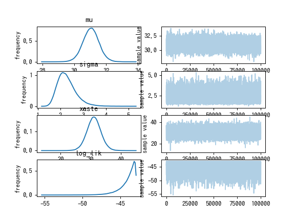
fit.plot()
plt.savefig("%s/%s1.png" % (dirname(__file__), basename(__file__)), dpi=90)
#plt.show()
sigma = pdata['sigma']
mu = pdata['mu']
var = sigma**2 #分散(variance)
cv = sigma / mu #変動係数(coefficient of variation)
prob = np.array([0.025, 0.05, 0.5, 0.95, 0.975])*100
desc = [ "", "EAP", "post.sd" ] + prob.tolist()
varinfo = [ "分散 ", np.mean(var), np.std(var) ] + np.percentile(var, prob).tolist()
cvinfo = [ "変動係数", np.mean(cv), np.std(cv) ] + np.percentile(cv, prob).tolist()
fmt = "{:^4}" + "{:>10.2f}" * (len(varinfo) - 1)
print("")
print(("{:^8}{:>10}{:>10}" + "{:>9.1f}%"*(len(varinfo)-3)).format(*desc))
print(fmt.format(*varinfo))
print(fmt.format(*cvinfo))実行の結果
Gradient evaluation took 1.5e-05 seconds
Gradient evaluation took 2.1e-05 seconds
Gradient evaluation took 2.5e-05 seconds
Gradient evaluation took 2.1e-05 seconds
1000 transitions using 10 leapfrog steps per transition would take 0.15 seconds.
Adjust your expectations accordingly!

1000 transitions using 10 leapfrog steps per transition would take 0.21 seconds.

Adjust your expectations accordingly!
1000 transitions using 10 leapfrog steps per transition would take 0.25 seconds.
1000 transitions using 10 leapfrog steps per transition would take 0.21 seconds.
Adjust your expectations accordingly!


Adjust your expectations accordingly!


Iteration:     1 / 21000 [  0%]  (Warmup)
Iteration:     1 / 21000 [  0%]  (Warmup)
Iteration:     1 / 21000 [  0%]  (Warmup)
Iteration:     1 / 21000 [  0%]  (Warmup)
Iteration:  1001 / 21000 [  4%]  (Sampling)
Iteration:  1001 / 21000 [  4%]  (Sampling)
Iteration:  1001 / 21000 [  4%]  (Sampling)
Iteration:  1001 / 21000 [  4%]  (Sampling)
Iteration:  3100 / 21000 [ 14%]  (Sampling)
Iteration:  3100 / 21000 [ 14%]  (Sampling)
Iteration:  3100 / 21000 [ 14%]  (Sampling)
Iteration:  3100 / 21000 [ 14%]  (Sampling)
Iteration:  5200 / 21000 [ 24%]  (Sampling)
Iteration:  5200 / 21000 [ 24%]  (Sampling)
Iteration:  5200 / 21000 [ 24%]  (Sampling)
Iteration:  7300 / 21000 [ 34%]  (Sampling)
Iteration:  7300 / 21000 [ 34%]  (Sampling)
Iteration:  5200 / 21000 [ 24%]  (Sampling)
Iteration:  7300 / 21000 [ 34%]  (Sampling)
Iteration:  9400 / 21000 [ 44%]  (Sampling)
Iteration:  9400 / 21000 [ 44%]  (Sampling)
Iteration:  9400 / 21000 [ 44%]  (Sampling)
Iteration:  7300 / 21000 [ 34%]  (Sampling)
Iteration: 11500 / 21000 [ 54%]  (Sampling)
Iteration: 11500 / 21000 [ 54%]  (Sampling)
Iteration: 11500 / 21000 [ 54%]  (Sampling)
Iteration: 13600 / 21000 [ 64%]  (Sampling)
Iteration: 13600 / 21000 [ 64%]  (Sampling)
Iteration:  9400 / 21000 [ 44%]  (Sampling)
Iteration: 13600 / 21000 [ 64%]  (Sampling)
Iteration: 15700 / 21000 [ 74%]  (Sampling)
Iteration: 15700 / 21000 [ 74%]  (Sampling)
Iteration: 15700 / 21000 [ 74%]  (Sampling)
Iteration: 17800 / 21000 [ 84%]  (Sampling)
Iteration: 11500 / 21000 [ 54%]  (Sampling)
Iteration: 17800 / 21000 [ 84%]  (Sampling)
Iteration: 19900 / 21000 [ 94%]  (Sampling)
Iteration: 17800 / 21000 [ 84%]  (Sampling)
Iteration: 19900 / 21000 [ 94%]  (Sampling)
Iteration: 21000 / 21000 [100%]  (Sampling)

 Elapsed Time: 0.019063 seconds (Warm-up)
               0.287619 seconds (Sampling)
               0.306682 seconds (Total)

Iteration: 13600 / 21000 [ 64%]  (Sampling)
Iteration: 21000 / 21000 [100%]  (Sampling)

 Elapsed Time: 0.019535 seconds (Warm-up)
               0.300162 seconds (Sampling)
               0.319697 seconds (Total)

Iteration: 19900 / 21000 [ 94%]  (Sampling)

Gradient evaluation took 5e-06 seconds
1000 transitions using 10 leapfrog steps per transition would take 0.05 seconds.
Adjust your expectations accordingly!


Iteration:     1 / 21000 [  0%]  (Warmup)
Iteration: 21000 / 21000 [100%]  (Sampling)

 Elapsed Time: 0.017516 seconds (Warm-up)
               0.329674 seconds (Sampling)
               0.34719 seconds (Total)

Iteration:  1001 / 21000 [  4%]  (Sampling)
Iteration: 15700 / 21000 [ 74%]  (Sampling)
Iteration:  3100 / 21000 [ 14%]  (Sampling)
Iteration: 17800 / 21000 [ 84%]  (Sampling)
Iteration:  5200 / 21000 [ 24%]  (Sampling)
Iteration: 19900 / 21000 [ 94%]  (Sampling)
Iteration:  7300 / 21000 [ 34%]  (Sampling)
Iteration: 21000 / 21000 [100%]  (Sampling)

 Elapsed Time: 0.019017 seconds (Warm-up)
               0.412707 seconds (Sampling)
               0.431724 seconds (Total)

Iteration:  9400 / 21000 [ 44%]  (Sampling)
Iteration: 11500 / 21000 [ 54%]  (Sampling)
Iteration: 13600 / 21000 [ 64%]  (Sampling)
Iteration: 15700 / 21000 [ 74%]  (Sampling)
Iteration: 17800 / 21000 [ 84%]  (Sampling)
Iteration: 19900 / 21000 [ 94%]  (Sampling)
Iteration: 21000 / 21000 [100%]  (Sampling)

 Elapsed Time: 0.019063 seconds (Warm-up)
               0.183481 seconds (Sampling)
               0.202544 seconds (Total)

Inference for Stan model: anon_model_6499076def106ab9bf01895c3ac67f18.
5 chains, each with iter=21000; warmup=1000; thin=1;
post-warmup draws per chain=20000, total post-warmup draws=100000.

          mean se_mean     sd   2.5%    25%    50%    75%  97.5%  n_eff   Rhat
mu       31.05  2.0e-3   0.52  30.02  30.71  31.04  31.38  32.07  69788    1.0
sigma     2.28  1.6e-3    0.4   1.65   1.99   2.22    2.5   3.22  65590    1.0
xaste    31.03  7.6e-3   2.38  26.32   29.5  31.03  32.57  35.74  98111    1.0
log_lik -44.03  5.5e-3   1.12 -47.04 -44.46 -43.68 -43.23 -42.94  41083    1.0
lp__    -24.84  5.2e-3   1.05 -27.68 -25.25 -24.51 -24.09 -23.82  41148    1.0

Samples were drawn using NUTS at Fri Jun  8 17:27:08 2018.
For each parameter, n_eff is a crude measure of effective sample size,
and Rhat is the potential scale reduction factor on split chains (at
convergence, Rhat=1).

               EAP   post.sd      2.5%      5.0%     50.0%     95.0%     97.5%
分散        5.34      2.02      2.72      2.97      4.93      9.10     10.39
変動係数      0.07      0.01      0.05      0.06      0.07      0.10      0.10